Statistical Tests for Random Number Generators
 Running statistical tests for randomness on a random number generator seems to be a bit of an
oxymoron. It’s random. If I generate ten numbers from 1 to 10,
 1-1-1-1-1-1-1-1-1-1 is just as
valid of a sequence as 6-2-6-7-9-1-3-5-8-8.
Statistical testing is really just a formalization of human intuition. If I flipped a coin 5 times and got all heads, we probably wouldn’t think anything of it. In more formal words, the probability of getting 5 heads in a row isn’t all that low, so we have no reason to reject the null hypothesis that the coin is fair. On the other hand, if we flipped the coin 20 times and got heads 19 of the 20 tosses, we would probably think something is up. The probability of getting 19 heads in 20 coin tosses is about a thousandth of a percent – really low. We have reasonable suspicion to think that the coin is weighted to give more heads than tails.
We apply the same logic with testing for random number generators. We make an assumption that the generator is a true random number generator and then try to prove our assumption wrong. If something seemingly odd happens, we conclude either “there is a reasonable probability that it happened just by chance/dumb luck” or “the probability of this happening just by chance/dumb luck is significantly low.”
When we test random number generators, we need to test for two main things: uniformity and independence. Uniformity simply means that the numbers are uniformly distributed. In other words, if we generate 100 random numbers from 1 to 10, we should see approximately ten 1s, ten 2s, ten 3s, and so on. As n increases, the closer the distribution comes to being uniform. Independence means that any and all prior outputs of the random number generator should have absolutely no effect on the next output. Do note that independence is the more important of the two. Uniformity can be fixed via a process called whitening. Nothing can fix a random number generator that doesn’t have independent outcomes.
Test 1: Monte Carlo Simulation of Pi
Let’s start out with a test that is really not the best for testing randomness. The perks are that it is very straightforward even to stats novices and the results are somewhat more exciting than a typical “pass/fail”. Let’s approximate Pi using a Monte Carlo Simulation.
Disclaimer: I’m not an art major nor could I be. You’re about to find out why.
We start out with this little piece of the first quadrant.
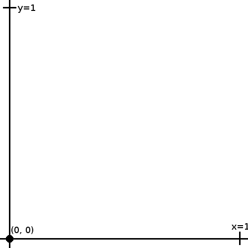
Next, we draw a 1×1 square from (0, 0) to (1, 1).
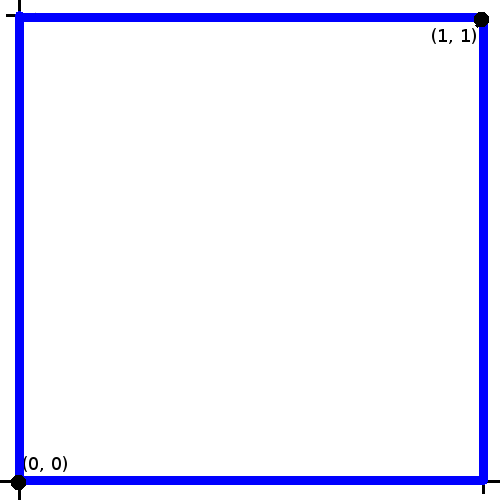
We then divide the square into two regions: those with a distance of less than or equal to 1 unit from the origin, and those with a distance greater than 1. You can draw a quartercircle as a dividing line. The quartercircle is centered at the origin with radius 1.
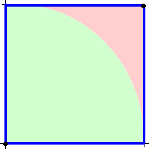
Finally, we generate a bunch of random points that lie within the square. We categorize these points on whether or not they lie within the green region.
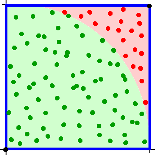
We then use a handy fact of random number generation; a good random number generator will uniformly distribute the points. This means that the ratio of the green points to the total number of points should approximately equal the radio of the area of the quartercircle to the area of the square. That’s pretty neat because we know the area of both of those. A square has an area of \(side^2\). Our side is length 1, so the area of the square is simply 1. A quartercircle has an area of \(\pi * radius^2 / 4\). Our radius is 1, so the area is \(\pi / 4\). Thus the number of generated points in the green region divided by the total number of points is approximately equal to \(\pi / 4\).
With a good random number generator, as \(n\) approaches infinity, four times the number of points in the green region divided by the total number of points approaches \(\pi\).
I created this method to test a random number generator using the method above.
    public boolean testPiEstimateMonteCarloSimulation(final int points, final double acceptedError) {
        startTimer();
        println("Running Monte Carlo Simulation");
        printLineSeparator();
        println(String.format("Approximating pi using %d points", points));
        int pointsWithinQuadrant = 0;
        for(int i = 0; i < points; i++) {
            double x = supplier.getAsDouble();
            double y = supplier.getAsDouble();
            if(Math.hypot(x, y) < 1)
                pointsWithinQuadrant++;
        }
        double pi = (4.0 * pointsWithinQuadrant) / points;
        println(String.format("Pi was calculated to be %f", pi));
        double percentDiff = (pi - Math.PI) / Math.PI;
        println(String.format("Percent difference between actual value is %f%%",
                percentDiff * 100.0));
        if(Math.abs(percentDiff) < acceptedError) {
            println(String.format("Calculated value is within accepted error of %.3f%%; "
                    + "test passed.", acceptedError * 100.0));
            finishTimer();
            return true;
        }
        println(String.format("Calculated value is not within accepted error of %.3f%%; "
                + "test failed.", acceptedError * 100.0));
        finishTimer();
        return false;
    }
Let’s see how the generator I created in another blog post squares up against the Middle Square Method (a bad generator) and the Java random implementation. Note that Java random uses a very similar algorithm as my random number generator, so we should expect similar results.
Running Monte Carlo Simulation - Middle Square Random
------------------------------------------------------------
Approximating pi using 10000000 points
Pi was calculated to be 3.192063
Percent difference between actual value is 1.606515%
Calculated value is not within accepted error of 0.020%; test failed.
Test executed in 7.705617 seconds


Running Monte Carlo Simulation - Linear Congruential Random
------------------------------------------------------------
Approximating pi using 10000000 points
Pi was calculated to be 3.141897
Percent difference between actual value is 0.009681%
Calculated value is within accepted error of 0.020%; test passed.
Test executed in 7.660834 seconds


Running Monte Carlo Simulation - java.util Random
------------------------------------------------------------
Approximating pi using 10000000 points
Pi was calculated to be 3.141030
Percent difference between actual value is -0.017923%
Calculated value is within accepted error of 0.020%; test passed.
Test executed in 8.150636 seconds
Pretty much as expected, the Middle Square Method fails and the other two pass.
Test 2: Generating Random Bitmaps
The next test I would like to talk about is surprisingly effective and straightforward. It tests a different aspect of random number generators than the previous test, independence.
We know that all pseudorandom number generators are not independent. This fact is simply characteristic for them. Pseudorandom number generators will always repeat their sequence of numbers after some number, \(n\). Because of this, we know that if we generate \(n + 1\) pseudorandom numbers. the last number will always be the same as the first, hence the assumption of independence is broken.
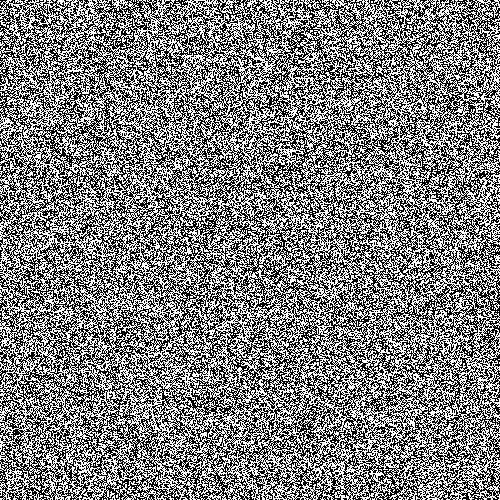
To perform this test, we simply generate a large random bitmap. To do that, for each pixel we use the random number generator to generate a true/false value – essentially a digital “coin flip.” If we get an output of true, we will color the pixel black. Otherwise, leave it white.
Here’s the cool part: once the image is generated, you get to perform the test! Open the generated image in your favorite image viewer and have a look. The image from a poor random number generator should have noticeable patterns. The image from a good random number generator should look something like an old television set with the coax cable unplugged.
Here’s the code I wrote for generating random bitmaps.
    public RenderedImage generateRandomBitmap(final int width, final int height) {
        startTimer();
        println("Generating Random Bitmap");
        printLineSeparator();
        println(String.format("Image size %dx%d", width, height));
        BufferedImage bi = new BufferedImage(width, height, BufferedImage.TYPE_BYTE_BINARY);
        Graphics2D g = bi.createGraphics();
        g.setColor(Color.WHITE);
        g.fillRect(0, 0, width, height);
        g.setColor(Color.BLACK);
        println("Generating image...");
        for(int x = 0; x < width; x++) {
            for(int y = 0; y < height; y++) {
                if(supplier.getAsDouble() < 0.5) {
                    g.fillRect(x, y, 1, 1);
                }
            }
        }
        finishTimer();
        return bi;
    }
Let’s check out some actual generated images. Here’s one from my linear congruential generator.
Compare that to the image from the Middle Square Method.
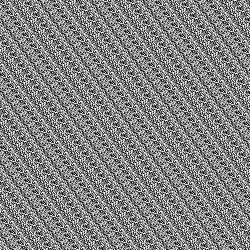
Clearly, there’s a pattern which implies that the random number generator isn’t all that great. In other words, the length of the sequence of random numbers before they start repeating is fairly small. Note that if you generate a large enough bitmap with pretty much any pseudorandom number generator and then stand far enough away so you can focus on a large portion of the image at once, you will see patterns in the bitmap. It’s simply characteristic of all non-“truely random” generators since they will all repeat after some amount of time.
Test 3: Chi-squared Goodness of Fit
The third test is a little more statistical and a little better test of randomness. Unfortunately, it’s also a little less visual and a little less glorious to talk about. We perform a chi-square goodness of fit test. First, uniformly generate a bunch of integers from let’s say 0 to 9. If we generate 1000, we expect to get 100 of each number. We expect to get around 10 sequences of each number occurring twice in a row. We expect to get around 1 sequence of each number occurring thrice in a row. We run the test for each of these scenarios. Our chi-square test statistic is computed by the formula:
\[\begin{align} \sum (observed - expected)^2 / expected \end{align}\]We have \(k-1\) degrees of freedom. K is equal to 10 since there are 10 counters we are comparing to their expected values. At a significance level of \(0.05\), we get a test statistic of \(19.023\). Accordingly, if any of our test statistics are greater than \(19.023\), we reject the null hypothesis that the random number generator is uniform and independent. Here’s my code for running a chi-squared goodness of fit test.
    public boolean testChiSquaredGoodnessOfFit(final int k, final int independenceDepth,
            final long n, final double critValue) {
        startTimer();
        println("Running Chi-Squared Goodness of Fit Test");
        printLineSeparator();
        IntSupplier intSupplier = () -> {
            return (int) (supplier.getAsDouble() * k);
        };
        println(String.format("Running test with k=%d, independenceDepth=%d, n=%d, critVal=%.3f",
                k, independenceDepth, n, critValue));
        int[] observed = new int[k];
        double expected = n / Math.pow(k, independenceDepth + 1);
        int independenceCounter = 0;
        int last = intSupplier.getAsInt();
        for(int i = 0; i < n; i++) {
            if(independenceCounter >= independenceDepth)
                observed[last]++;
            int next = intSupplier.getAsInt();
            if(next == last)
                independenceCounter++;
            else
                independenceCounter = 0;
            last = next;
        }
        double chiSquared = 0.0;
        for(int i = 0; i < k; i++) {
            chiSquared += (observed[i] - expected) * (observed[i] - expected) / expected;
        }

        println(String.format("Chi-squared=%f", chiSquared));
        if(chiSquared < critValue) {
            println(String.format("Chi-squared is less than the critical value of %.3f; test pa"
                    + "ssed.", critValue));
            finishTimer();
            return true;
        }
        println(String.format("Chi-squared is greater than the critical value of %.3f; test fai"
                + "led.", critValue));
        finishTimer();
        return false;
    }
Let’s check out the results for a variety of parameters.
Running Chi-Squared Goodness of Fit Test - Middle Square Random
------------------------------------------------------------
Running test with k=10, independenceDepth=0, n=100000000, critVal=19.023
Chi-squared=124667.064611
Chi-squared is greater than the critical value of 19.023; test failed.
Test executed in 1.240647 seconds


Running Chi-Squared Goodness of Fit Test - Linear Congruential Random
------------------------------------------------------------
Running test with k=10, independenceDepth=0, n=100000000, critVal=19.023
Chi-squared=7.511756
Chi-squared is less than the critical value of 19.023; test passed.
Test executed in 0.781947 seconds


Running Chi-Squared Goodness of Fit Test - java.util Random
------------------------------------------------------------
Running test with k=10, independenceDepth=0, n=100000000, critVal=19.023
Chi-squared=3.883786
Chi-squared is less than the critical value of 19.023; test passed.
Test executed in 3.458994 seconds


Running Chi-Squared Goodness of Fit Test - Middle Square Random
------------------------------------------------------------
Running test with k=10, independenceDepth=1, n=100000000, critVal=19.023
Chi-squared=431373.006028
Chi-squared is greater than the critical value of 19.023; test failed.
Test executed in 1.135735 seconds


Running Chi-Squared Goodness of Fit Test - Linear Congruential Random
------------------------------------------------------------
Running test with k=10, independenceDepth=1, n=100000000, critVal=19.023
Chi-squared=5.967571
Chi-squared is less than the critical value of 19.023; test passed.
Test executed in 0.696090 seconds


Running Chi-Squared Goodness of Fit Test - java.util Random
------------------------------------------------------------
Running test with k=10, independenceDepth=1, n=100000000, critVal=19.023
Chi-squared=5.031364
Chi-squared is less than the critical value of 19.023; test passed.
Test executed in 3.085213 seconds


Running Chi-Squared Goodness of Fit Test - Middle Square Random
------------------------------------------------------------
Running test with k=10, independenceDepth=3, n=100000000, critVal=19.023
Chi-squared=862834.392100
Chi-squared is greater than the critical value of 19.023; test failed.
Test executed in 1.319469 seconds


Running Chi-Squared Goodness of Fit Test - Linear Congruential Random
------------------------------------------------------------
Running test with k=10, independenceDepth=3, n=100000000, critVal=19.023
Chi-squared=7.317500
Chi-squared is less than the critical value of 19.023; test passed.
Test executed in 1.538459 seconds


Running Chi-Squared Goodness of Fit Test java.util Random
------------------------------------------------------------
Running test with k=10, independenceDepth=3, n=100000000, critVal=19.023
Chi-squared=13.673000
Chi-squared is less than the critical value of 19.023; test passed.
Test executed in 3.162882 seconds
It’s not exactly a surprise that Linear Congruential Random and java.util Random pass while Middle Square Random fails atrociously. I think you’re starting to see a pattern here.
Test 4: Entropy Test Via Compression Ratio
Last but not least, we test the entropy by seeing the zip compression ratio achieved. Once upon a time, a really smart guy named Phil Katz spent a long time creating the zip file format. It employs a very intelligent algorithm designed to search for patterns in the bits of a binary file. After finding these patterns, it encodes them. The result is that the file is comressed, sometimes dramatically depending on the content. Many modern file file formats (like .docx and .xlsx) actually are a zip file containing a bunch of .xml files with templates and content Don’t believe me? Make a Word document, type something, save it, rename the file from .docx to .zip, and open it up! So we’ve established that zip compression works more or less by finding order. Order turns out to be the opposite of randomness, in the file. An ASCII character is one byte, or 8 bits. Generally, in the English language you’ll see 1-2 bits of randomness (more formally called entropy) per character. That means that when a .txt file containing English text is compressed, you’ll see a compression ratio (uncompressed size / compressed size) in the range of 4 to 8. When the text is randomly generated, you would think that you would see a compression ratio near 1 since each and every bit is random. ASCII characters happen to have one parity bit though so for every generated character we get only 7 bits of entropy, not 8. Because of this, our “perfect” compression ratio is about 8/7ths, or about 1.14. Let’s say when we test our generator’s compression ratio, a ratio of 1.15 or less is passing.
Here’s the code:
    public boolean testEntropyWithZipRatio(final long characters,
            final double passingCompressionRatio) {
        startTimer();
        println("Running Zip Compression Ratio Entropy Test");
        printLineSeparator();
        println(String.format("Running test with %d bytes and comparing compression ratio against"
                + " critical value of %.3f", characters, passingCompressionRatio));
        Supplier<Character> charSupplier = () -> {
            return (char) (supplier.getAsDouble() * 128); // random ASCII char
        };

        try {
            final File zipFile = File.createTempFile("tmp", ".zip");
            final File txtFile = File.createTempFile("tmp", ".txt");
            final ZipOutputStream zos = new ZipOutputStream(new FileOutputStream(zipFile));
            zos.putNextEntry(new ZipEntry("chars.txt"));
            OutputStreamWriter zipWriter = new OutputStreamWriter(zos);
            FileWriter txtWriter = new FileWriter(txtFile);
            for(int i = 0; i < characters; i++) {
                char c = charSupplier.get();
                zipWriter.write(c);
                txtWriter.write(c);
            }
            zipWriter.close();
            txtWriter.close();
            long zipSize = Files.size(zipFile.toPath());
            long txtSize = Files.size(txtFile.toPath());
            println(String.format("Uncompressed size: %d bytes", txtSize));
            println(String.format("Compressed size: %d bytes", zipSize));
            double ratio = (double) txtSize / zipSize;
            println(String.format("Compression ratio: %f", ratio));
            if(ratio < passingCompressionRatio) {
                println("Compression ratio is less than critical value; test passed.");
                finishTimer();
                return true;
            }
        } catch(IOException e) {
            e.printStackTrace();
            return false;
        }
        println("Compression ratio is greater than critical value; test failed.");
        finishTimer();
        return false;
    }
How did our three generators square up in the zip test?
Running Zip Compression Ratio Entropy Test - Middle Square Random
------------------------------------------------------------
Running test with 33554432 bytes and comparing compression ratio against critical value of 1.150
Uncompressed size: 33596010 bytes
Compressed size: 201094 bytes
Compression ratio: 167.066198
Compression ratio is greater than critical value; test failed.
Test executed in 3.745677 seconds


Running Zip Compression Ratio Entropy Test - Linear Congruential Random
------------------------------------------------------------
Running test with 33554432 bytes and comparing compression ratio against critical value of 1.150
Uncompressed size: 33554432 bytes
Compressed size: 29445850 bytes
Compression ratio: 1.139530
Compression ratio is less than critical value; test passed.
Test executed in 4.702422 seconds


Running Zip Compression Ratio Entropy Test - java.util Random
------------------------------------------------------------
Running test with 33554432 bytes and comparing compression ratio against critical value of 1.150
Uncompressed size: 33554432 bytes
Compressed size: 29445771 bytes
Compression ratio: 1.139533
Compression ratio is less than critical value; test passed.
Test executed in 4.369030 seconds
Wow! This test is where the Middle Square Method really shows it’s true colors as an inferior random number generator. Both my linear congruential generator and java.util Random have compression ratios right at the limit of 8/7ths. The Middle Square Method’s is an astounding 167!
As you can see, there’s a wide variety of ways to test random number generators. I’ve presented four of them each with their own merits. Feel free to use them as you choose and I hope they serve you well; perhaps you’ll be the person who creates the latest quick, efficient, and effective pseudorandom number generating algorithm!