Animal Crossing: Forecasting Turnip Prices with Bayesian Inference

Introduction

Turnips are bitter, smelly, generally disgusting root vegetables that I imagine only two-pack-a-day smokers who have burned off their taste buds can bear to eat. Despite that, during these strange times as we all sit in our homes trying to build a better life for ourselves in the virtual island paradise that is Animal Crossing, the Stalk Market for buying and selling turnips has captured many of our imaginations. With the real market sinking and our 401Ks making it look more and more likely we’ll never be able to retire, many of us have turned to this virtual market in the hopes of at least capturing a consolation prize of becoming a bellionaire.

Here’s how the Stalk Market works: on Sunday Daisy Mae strolls onto your island and will sell turnips during the morning at a price between 90 and 110 bells per turnip. You can then sell the turnips you purchased at Nook’s Cranny for whatever the market price happens to be. This price changes twice per day: once each morning and once at noon. Any turnips not sold by the next Sunday will spoil and become worthless.

As someone working in the trading industry, as soon as my fiancée told me about Animal Crossing’s Stalk Market, my thoughts immediately went to “how can I model and/or forecast the prices?” After a bit of quick research, the internet taught me that the prices are generated at the beginning of the week according to a few randomized patterns.

Like many people playing the Stalk Market, I then came across the numerous online Turnip Calculators. When looking into their methodology, they all pointed to one place: a snippet of code from a Gibraltarian university student in Scotland who reverse engineered the turnip price-generating logic.¹

Studying the code

Studying the code, I confirmed a couple things. Your “buy price” (I’ll call it “base price” from now on) is indeed randomly chosen from 90-110 bells, and one of four patterns is chosen each week.

1. Up-Down-Up-Down
2. Big Spike
3. Decreasing
4. Small Spike

Which pattern is chosen depends mainly on whether you’re a new turnip buyer and what last week’s pattern was. Each of the four patterns themselves are also randomized in a constrained manner. As shown in Appendix B, over the long run your island will spend about equal time in each of the four patterns.

Up-Down-Up-Down

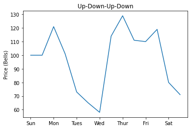
With the Up-Down-Up-Down pattern, the price sort of bounces around near the base price. Some other people have called this a “random” pattern, but I refrain from using that term because it isn’t really just a week of random prices: there is some structure to it. The exact structure of the pattern can be seen in the below table.

Phase	Length	Description
A	0-3 days	90-140% of base price
B	1-1.5 days	60-80% of base price, then decreasing by 4-10% of base price
C	0.5-3.5 days	90-140% of base price
D	1-1.5 days	60-80% of base price, then decreasing by 4-10% of base price
E	0-3 days	90-140% of base price

Note: Phases A+C+E = 3.5 days and Phases B+D = 2.5 days.

Big Spike

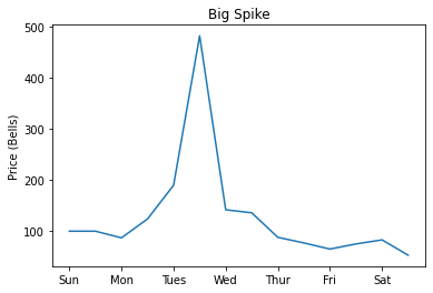
The Big Spike pattern, as its name implies, is the one you really would like to have every week. The week starts and ends with a period of decreasing prices. Sandwiched in the middle of those periods lies a big spike of up to 6x the base price.

Phase	Length	Description
A	0.5-3.5 days	85-90% of base price, then decreasing by 3-5% of base price
B	1 day	90-140% of base price, then 140-200% of base price
C	0.5 days	200-600% of base price
D	1 day	140-200% of base price, then 90-140% of base price
E	0-3 days	40-90% of base price

Note: Phases A+E = 3.5 days.

Decreasing

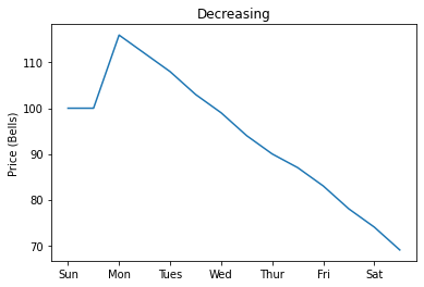
The Decreasing pattern is the worst of the four patterns. Over the entire week, the prices gradually decreases.

Phase	Length	Description
A	6 days	85-90% of base price, then decreasing by 3-5% of base price

Small Spike

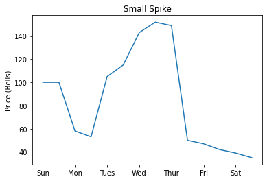
The Small Spike pattern is similar to the Big Spike pattern but with a few notable differences. The peak is obviously much smaller (up to 2x base price), the timelines for when the peak happens are a bit different, and the initial Monday morning price is likely to be lower.

Phase	Length	Description
A	0-3.5 days	40-90% of base price, then decreasing by 3-5% of base price
B	1 day	90-140% of base price
C	0.5 days	between 140% of base price and the Phase D price
D	0.5 days	140-200% of base price
E	0.5 days	between 140% of base price and the Phase D price
F	0-3.5 days	40-90% of base price, then decreasing by 3-5% of base price

Note: Phases A+F = 3.5 days.

Forecasting Prices

My first idea for forecasting the prices was to brute force all of the possible patterns for a week and pattern match the prices seen early in the week to get a probabilistic forecast for the remainder of the week, but that method turned out to be a bust. I’ve elaborated a bit more on it in Appendix A if you’re interested.

The method I ended up settling on is extracting the probabilities from the code and relying on Bayesian Inference². Bayes’ Theorem states

\[P(B|A) = \frac{P(A|B)P(B)}{P(A)}\]

That is, the probability of \(B\) happening given we know \(A\) has happened is the probability that \(A\) happens given \(B\) has happened multiplied by the probability ratio of \(B\) and \(A\). We can use this theorem to formulate useful expressions for our turnip pricing. For example,

\[P(\text{Big Spike}|\text{Mon. AM price of 94 bells}) = \frac{P(\text{Mon. AM price of 94 bells} | \text{Big Spike})P(\text{Big Spike})}{P(\text{Mon. AM price of 94 bells})}\]

To begin with, we need to know what pattern we are in. The generating distribution is shown in the following flowchart.

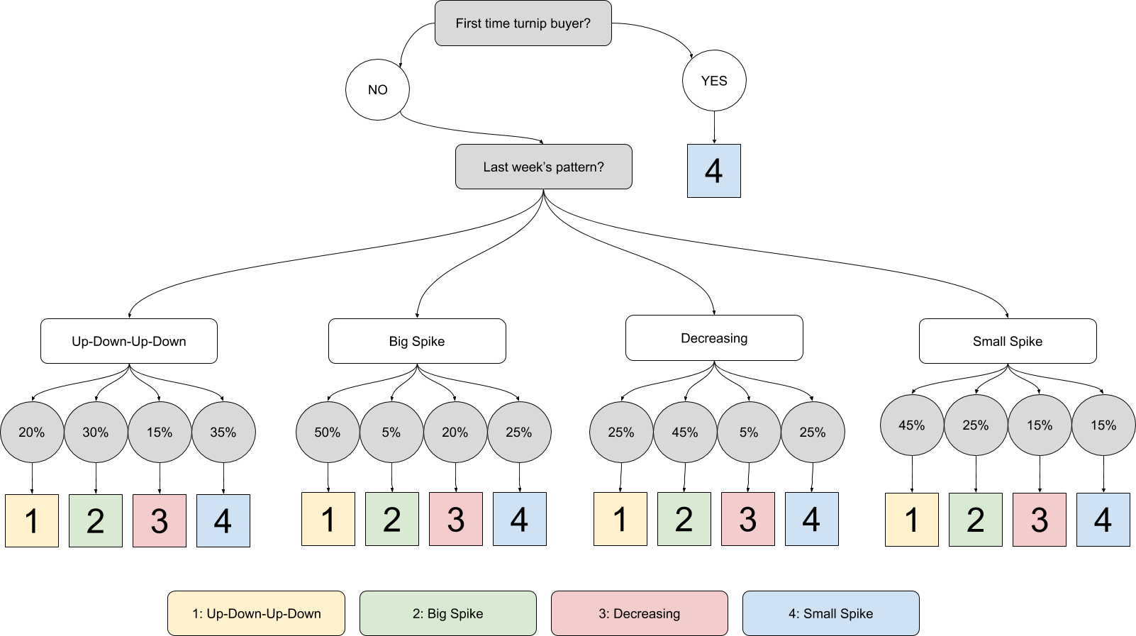
Last week’s pattern can also be thought of as a random variable - if you aren’t sure whether you were in an Up-Down-Up-Down pattern or a Small Spike pattern, you can just assign these probabilities either via guessing or via maximum likelihood estimation. If you have absolutely no idea, you can model the pattern as a Markov Process³ and compute the stationary distribution (see Appendix B). Multiplying our last week probabilities by each pattern’s “next pattern” probability distribution yields our Bayesian priors for the current week’s pattern (in the above expression, the “prior” is \(P(\text{Big Spike})\)).

Examples

The math can be a bit difficult to visualize, so let’s go through a few concrete examples using real prices from the island I live on.

Week of April 26

On the week of April 26, the previous week had a Small Spike pattern. From the flow chart, this gives the following priors (note, I use \(P_1\) for the probability of Up-Down-Up-Down, \(P_2\) for the probability of Big Spike, and so on).

\[P_1 = 0.45 \\ P_2 = 0.25 \\ P_3 = 0.15 \\ P_4 = 0.15\]

The turnip buy price was 106 bells, and on Monday morning, the price of turnips was 94 bells. Because the patterns work by scaling the base price, it’s more convenient to look at this as a percentage of the base price. Because the code used rounds results upwards, I also subtract \(0.5\) from my price since that’s actually the “mean” price before the code rounds it up.

\[X = \frac{93.5}{106} = 88.21\%\]

Straight away, we can observe a few things.

1. We cannot be in Up-Down-Up-Down because the \(88.21\%\) of base price is impossible on day 1.
2. We are much more likely to be in Decreasing or Big Spike than Little Spike because getting \(88.21\%\) is much more likely for a uniform random variable between \(0.85\) and \(0.9\) than one between \(0.4\) and \(0.9\).

To begin with, we compute the tailed conditional probability of getting such a price, given we’re in a specific pattern. Note that for Small Spike we need to multiply by \(\frac{7}{8}\) because there’s a \(\frac{1}{8}\) chance that “Phase A” in that pattern is 0 days long (and the probability is 0 if we start in “Phase B”).

\[P(\text{Monday's price}|\text{Up-Down-Up-Down}) = 0 \\ P(\text{Monday's price}|\text{Big Spike}) = 1 - \frac{0.8821 - 0.85}{0.9 - 0.85} = 0.3585 \\ P(\text{Monday's price}|\text{Decreasing}) = 1 - \frac{0.8821 - 0.85}{0.9 - 0.85} = 0.3585 \\ P(\text{Monday's price}|\text{Small Spike}) = \frac{7}{8} \cdot (1 - \frac{0.8821 - 0.4}{0.9 - 0.4}) = 0.0314\]

To find the tail probability of Monday’s price in general, we apply the formula

\[P(\text{Monday's price}) = \sum_{\text{pattern}} P(\text{pattern})P(\text{Monday's price}|\text{pattern})\]

In our case, this yields

\[P(\text{Monday's price}) = 0.45 \cdot 0 + 0.25 \cdot 0.3585 + 0.15 \cdot 0.3585 + 0.15 \cdot 0.0314 = 0.1481\]

Applying Bayes’ Theorem to each of the non-zero probability patterns gives the following results.

Big Spike:

\(P(\text{Big Spike}|\text{Monday's price}) = \frac{0.3585 \cdot 0.25}{0.1481} = 60.51\%\)

Decreasing:

\(P(\text{Decreasing}|\text{Monday's price}) = \frac{0.3585 \cdot 0.15}{0.1481} = 36.31\%\)

Small Spike:

\(P(\text{Small Spike}|\text{Monday's price}) = \frac{0.0314 \cdot 0.15}{0.1481} = 3.18\%\)

Hence, we’re likely in a Big Spike pattern. These probabilities then become the Bayesian priors for the next iteration of our pattern estimation when Nook’s Cranny releases the next turnip price. In the next example we’ll go into that in more detail together.

Over the following day, here’s what the prices were.

Day	AM Price	PM Price
04/26 (Sunday)	106
04/27 (Monday)	94	91
04/28 (Tuesday)	131

From this set of prices, we know we can no longer be in the Decreasing pattern. We can still be in either Big Spike or Small Spike, but it’s much more likely to be Big Spike. The next price was in the \(140-200\%\) of base price range, confirming that we were in a big spike pattern. As expected, we saw the spike the following morning (of 432 bells).

Week of May 3

On the week of May 3, the previous week had a Big Spike pattern. From the flow chart, this gives the following priors.

\[P_1 = 0.50 \\ P_2 = 0.05 \\ P_3 = 0.20 \\ P_4 = 0.25\]

The turnip buy price was 101 bells, and on Monday morning, the price of turnips was 88 bells. Again, calculating the percentage of the base price, we have

\[X = \frac{87.5}{101} = 86.63\%\]

This again intuitively means we cannot be in Up-Down-Up-Down, and we are most likely in either Big Spike or Decreasing (but from the flowchart, getting Big Spike twice in a row is unlikely, so it’s probably Decreasing). We then get the following probabilities.

\[P(\text{Monday's price}|\text{Up-Down-Up-Down}) = 0 \\ P(\text{Monday's price}|\text{Big Spike}) = 1 - \frac{0.8663 - 0.85}{0.9 - 0.85} = 0.3260 \\ P(\text{Monday's price}|\text{Decreasing}) = 1 - \frac{0.8663 - 0.85}{0.9 - 0.85} = 0.3260 \\ P(\text{Monday's price}|\text{Small Spike}) = \frac{7}{8} \cdot (1 - \frac{0.8663 - 0.4}{0.9 - 0.4}) = 0.0674\]

In computing the probability of having such a price on Monday, we have

\[P(\text{Monday's price}) = 0.50 \cdot 0 + 0.05 \cdot 0.3260 + 0.20 \cdot 0.3260 + 0.25 \cdot 0.0674 = 0.0984\]

Applying Bayes’ Theorem to each of the non-zero probability patterns gives the following results.

Big Spike:

\(P(\text{Big Spike}|\text{Monday's price}) = \frac{0.3260 \cdot 0.05}{0.0984} = 16.58\%\)

Decreasing:

\(P(\text{Decreasing}|\text{Monday's price}) = \frac{0.3260 \cdot 0.20}{0.0984} = 66.29\%\)

Small Spike:

\(P(\text{Small Spike}|\text{Monday's price}) = \frac{0.0674 \cdot 0.25}{0.0984} = 17.13\%\)

So, sadly, we’re probably in a Decreasing pattern. When the afternoon prices came in, our prices for the week looked like this.

Day	AM Price	PM Price
05/03 (Sunday)	101
05/04 (Monday)	88	83

To calculate the probabilities after the next price came in, we simply iterate. We use the probabilities just calculated as our new priors. The only way we can be in Big Spike or Small Spike is if we are still in the beginning decreasing part of the pattern. The rest of the math actually becomes a bit easier. We only need to compute the probability of such an event happening given we are in a given pattern and already saw Monday’s price.

\[P(\text{Tuesday's price}|\text{Big Spike}) = \frac{6}{7} \\ P(\text{Tuesday's price}|\text{Decreasing}) = 1 \\ P(\text{Tuesday's price}|\text{Small Spike}) = \frac{6}{7}\]

Then, computing the probability of Tuesday’s price, we have

\[P(\text{Tuesday's price}) = 0.1658 \cdot \frac{6}{7} + 0.6629 \cdot 1 + 0.1713 \cdot \frac{6}{7} = 0.9518\]

Again, applying Bayes’ Theorem, we have the following probabilities.

Big Spike:

\(P(\text{Big Spike}|\text{Tuesday's price}) = \frac{6}{7} \cdot \frac{0.1658}{0.9518} = 14.93\%\)

Decreasing:

\(P(\text{Decreasing}|\text{Tuesday's price}) = 1 \cdot \frac{0.6629}{0.9518} = 69.64\%\)

Small Spike:

\(P(\text{Small Spike}|\text{Tuesday's price}) = \frac{6}{7} \cdot \frac{0.1713}{0.9518} = 15.43\%\)

So, this next day’s data as you would expect only increased the likelihood that we are in the Decreasing pattern. The following days the prices continued decreasing and we were indeed in the Decreasing pattern. When this happens, the best thing you can really hope to do is to sell your turnips on a friend’s island.

Conclusion

Though you’d never want to eat a turnip, it’s understandable to want to forecast their prices in Animal Crossing: New Horizons. In just a few weeks, I’ve already made a fortune in the stalk market. With a bit of modeling, you too can forecast the turnip price patterns with great accuracy. If modeling turnip prices brings us together in these trying times, then I’m all for it. Please leave a comment with any thoughts or questions.

Appendix A: Brute Force Computing the Patterns

I’ve spent quite a bit of time studying how computers generate random numbers and I immediately recognized the algorithm used in the Switch random library as the Mersenne Twister⁴, which is generally thought to be a pretty good random number generator. Computers naturally produce deterministic outputs, so in order to produce “random” numbers, they “seed” an algorithm with some value (often in cases like this a timestamp is used) and from there the algorithm will produce a long (but repeating) and ideally difficult to predict sequence of numbers.

The Switch random library seeds with a 32-bit value so there are around 4 billion possible sequences. With 4 possible patterns to elaborate, that makes about 16 billion sequences to compute. I began down the path of writing some code to compute these sequences on a GPU (GPUs are much quicker at this sort of parallel computation than CPUs). I completed writing code for the Small Spike pattern and determined on my computer it would take a couple hours to compute the 4 billion sequences.

It was about that time that I read a tweet that made me realize that this methodology was flawed. Though it only accepts a 32-bit seed, the random number generator keeps 128-bits of state. The single random number generator is also shared for the entire game, not just for the turnip price calculation. Because of that, it’s impossible to know how calls to the random number generator were made before the turnip-pricing code is run. This essentially introduces another dimension and changes our 16 billion sequences to a much, much larger number that would make elaborating the patterns on my computer take more than my lifetime (and even if I could, just navagating the resulting dataset would be very cumbersome since it would likely be terabytes large at best).

That’s not to say solving the problem is impossible – these are the kinds of problems that government hackers tackle all the time. Obviously, with more computation resources than my home computer, the time to compute would be greatly reduced. The Mersenne Twister algorithm used could be analyzed to find mathematical weaknesses. The dimension could be reduced using heuristics (for example since the random number generator is seeded with the system time, there’s only a small range of seeds that could have been used for the initial seeding). I would do these things… but frankly they are all above my mental ability, financial ability, give-a-damn, or some combination of the three. Let’s chalk it up as “future work” and call it a day.

Appendix B: Computing the Pattern Stationary Distribution

From the flowchart in our “Forecasting Prices” section, we can build the following transition matrix.

\[P = \begin{bmatrix} 0.2 & 0.3 & 0.15 & 0.35 \\ 0.5 & 0.05 & 0.2 & 0.25 \\ 0.25 & 0.45 & 0.05 & 0.25 \\ 0.45 & 0.25 & 0.15 & 0.15 \end{bmatrix}\]

This yields the following equations

\[\pi_1 = 0.2 \pi_1 + 0.3 \pi_2 + 0.15 \pi_3 + 0.35 \pi_4 \\ \pi_2 = 0.5 \pi_1 + 0.05 \pi_2 + 0.2 \pi_3 + 0.25 \pi_4 \\ \pi_3 = 0.25 \pi_1 + 0.45 \pi_2 + 0.05 \pi_3 + 0.25 \pi_4 \\ \pi_4 = 0.45 \pi_1 + 0.25 \pi_2 + 0.15 \pi_3 + 0.15 \pi_4 \\\]

where \(\pi_n\) represents the probability of us being in pattern \(n\) at some arbitrary point in time. We also have the additional constraint that the sum of the stationary probabilities must add up to one. Thus,

\[\pi_1 + \pi_2 + \pi_3 + \pi_4 = 1\]

If we solve this system of five equations for the four unknown variables, we end up with

\[\pi_1 = 0.25 \\ \pi_2 = 0.25 \\ \pi_3 = 0.25 \\ \pi_4 = 0.25 \\\]

Thus, over the long run, one can expect to spend about one-fourth of the time in each of the four patterns.

References